
Expected Goals (xG) for Football Betting: Using Statistics to Win
 Available in US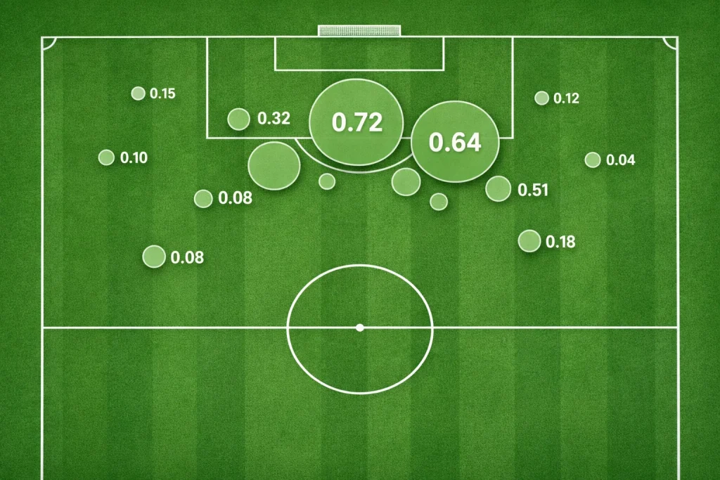
Expected Goals has transformed football analysis from subjective opinion to quantified performance measurement. While traditional statistics count shots without distinguishing a tap-in from a 30-yard speculative effort, xG assigns probability values based on historical conversion rates from similar positions and situations. A penalty receives approximately 0.78 xG (78% conversion rate historically); a tight-angle shot from 25 metres might receive 0.03 xG. Summing these probabilities across a match reveals how many goals a team “should” have scored based on the quality of chances created — often telling a completely different story than the actual scoreline.
For bettors, xG’s power lies in identifying when results don’t match underlying performance. Teams consistently outperforming their xG are likely to regress — their finishing luck will eventually normalise. Teams underperforming their xG are creating quality chances but not converting — positive regression likely awaits. Bookmakers increasingly incorporate xG into their models, but markets still react strongly to actual results, creating opportunities for bettors who look beyond scorelines to underlying chance quality.
How Expected Goals Is Calculated
xG models assign probability values to shots based on factors that historically affect conversion rates. While different providers (Opta, StatsBomb, Understat, FBref) use slightly varying methodologies, core factors remain consistent.
Distance from goal is the most significant factor. Shots from closer range convert more frequently than distant efforts. A shot from 6 metres has dramatically higher xG than one from 25 metres, reflecting the simple geometry of having more goal to aim at and less reaction time for the goalkeeper.
Angle to goal affects available target area. Shots from central positions have the full goal width available; shots from tight angles see most of the goal blocked by the near post and goalkeeper positioning. A chance from directly in front of goal receives higher xG than one from the same distance but near the touchline.
Shot type matters significantly. Shots with the foot generally convert at higher rates than headers, which are harder to direct accurately. One-on-one situations receive elevated xG values reflecting the advantageous positioning. Volleys and half-volleys have their own conversion profiles.
Assist type influences chance quality. A square ball across the six-yard box creates higher xG chances than a hopeful cross into a crowded penalty area. Through balls behind the defence create better opportunities than passes requiring the attacker to create their own angle.
Defensive pressure affects conversion rates. Shots with defenders blocking the line or closing quickly convert less frequently than uncontested efforts. Some advanced models incorporate defender positioning and goalkeeper location.
Game situation provides context. Penalties have fixed xG (approximately 0.78). Free kicks, corners, and open-play chances have different baseline conversion rates. Counter-attacks often create higher-xG chances than set-piece situations.
xG vs Actual Goals: Finding Regression Opportunities
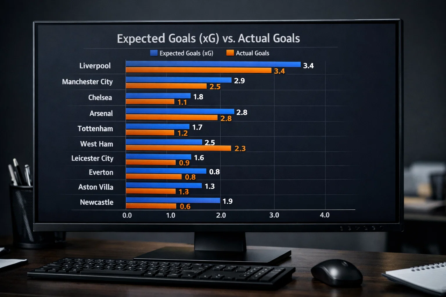
The core betting application of xG lies in identifying teams whose results don’t match their underlying performance. The principle is regression to the mean — over sufficient time, actual goals tend to converge toward expected goals.
Overperforming teams score more goals than their xG suggests. This might indicate exceptional finishing ability, but more often reflects luck — shots going in that normally wouldn’t. A team with 15 goals from 10 xG has been clinical or fortunate; either way, sustaining that conversion rate is improbable. These teams are candidates for “against” betting or unders.
Underperforming teams score fewer goals than their xG suggests. They’re creating quality chances but not converting — missing sitters, hitting woodwork, facing inspired goalkeepers. Regression suggests future goal-scoring improvement. These teams are candidates for backing or overs.
Rolling averages matter more than single matches. A team might have 3.0 xG but score 0 in one match through sheer bad luck. Single-match xG can mislead. But a team consistently generating 2.0 xG per match while only scoring 1.0 over ten matches reveals a genuine conversion problem likely to correct.
Calculate the xG difference (actual goals minus xG) over rolling periods. Teams with strongly positive differences (+5 or more over 10 matches) are overperforming and likely to regress downward. Teams with strongly negative differences (-5 or more) are underperforming and likely to regress upward.
Using xG Against (xGA) for Defensive Assessment
While xG measures attacking quality, xGA (expected goals against) measures defensive vulnerability — the quality of chances a team concedes.
Low xGA indicates strong defensive performance. The team isn’t allowing opponents quality shooting opportunities, whether through excellent defending, disciplined positioning, or controlling possession away from dangerous areas. Low xGA teams are genuinely difficult to score against.
High xGA indicates defensive weakness. The team concedes numerous quality chances even if they don’t all convert. A team conceding 8 goals from 15 xGA has been fortunate; their defence is leaking chances that will eventually be punished.
xGA regression works identically to xG regression. Teams significantly outperforming their xGA (conceding fewer goals than expected) will likely concede more in future. Teams underperforming xGA (conceding more than expected) may tighten up as statistical variance normalises.
Combined xG and xGA analysis reveals overall team quality. Strong teams generate high xG while allowing low xGA. Weak teams show the inverse pattern. Mid-table teams often cluster around league averages for both metrics.
Expected Points (xPTS) for League Analysis
Expected Points extends xG logic to match outcomes, estimating how many points a team “should” have accumulated based on their underlying performances rather than actual results.
xPTS models simulate thousands of match outcomes based on each team’s xG in each match, calculating average points across simulations. A team that won 1-0 despite being outplayed (opponent had 2.5 xG to their 0.8 xG) might receive only 0.5 xPTS despite earning 3 actual points.
League table vs xPTS table comparison reveals overperforming and underperforming teams. A team sitting 5th in the actual table but 12th in xPTS has been fortunate — their results exceed their underlying performance. Conversely, a team in 14th actual but 8th xPTS has been unlucky and may climb.
Outright betting applications emerge from xPTS analysis. If bookmakers price teams based partly on actual league position, teams with better xPTS than actual position may offer value in futures markets. Their underlying performances suggest better results should follow.
Practical Applications for Betting Markets
xG analysis applies across multiple betting markets, each requiring slightly different approaches.
Match winner markets: When a team with strong xG record faces an opponent who has been conceding high xGA, the attacking team has genuine value — quality chance creation meets defensive vulnerability. Conversely, backing teams simply because they’ve won recent matches (potentially through luck) ignores whether their performances justify the results.
Over/Under goals markets: Add both teams’ xG per game averages for expected match total. If Team A averages 1.8 xG and Team B averages 1.5 xG, expect approximately 3.3 total xG. Compare this estimate against bookmaker totals lines. If the line is 2.5 and you estimate 3.3 expected goals, overs offers potential value.
Both Teams to Score (BTTS): Combine xG (attacking quality) with opponent xGA (defensive vulnerability). If both teams generate reasonable xG and both concede reasonable xGA, BTTS becomes more probable. If one team generates minimal xG while their opponent has excellent defensive xGA, BTTS No gains probability.
Asian Handicap markets: xG differential (team xG minus team xGA) indicates expected goal difference per match. Teams with positive xG differential should, over time, win by margins that cover Asian handicap lines. This helps identify value on handicap markets where bookmakers might be reacting to actual results rather than underlying performances.
Live betting: Real-time xG during matches (available from some data providers) reveals whether the scoreline reflects match flow. A team losing 1-0 but dominating with 2.5 xG to 0.3 xGA represents potential live betting value — their performance suggests goals should follow.
Related Metrics: xA, Post-Shot xG, and xGOT
Expected Goals spawned related metrics that provide additional analytical depth.
Expected Assists (xA) measures pass quality independent of whether the recipient scored. A perfectly weighted through ball that creates a 0.6 xG chance earns 0.6 xA for the passer, regardless of whether the shot was converted. xA helps identify creative players and teams generating quality chances.
Post-Shot xG (PSxG) incorporates shot placement — where the shot was aimed, not just where it was taken from. A shot from 15 metres aimed at the top corner has higher PSxG than one aimed straight at the goalkeeper from the same position. PSxG helps separate shooting skill from chance creation.
xG On Target (xGOT) measures goalkeeper performance by evaluating the quality of shots they face versus shots they save. A goalkeeper conceding 20 goals from 25 xGOT on target has been above average; one conceding 25 goals from 20 xGOT has underperformed expected save rates.
Limitations and Caveats

xG is powerful but imperfect. Understanding its limitations prevents over-reliance.
Models vary between providers. Opta, StatsBomb, Understat, and others use different methodologies producing different xG values for identical shots. Don’t compare xG figures across providers; choose one source and use it consistently.
xG doesn’t capture everything. Player skill, team tactics, weather conditions, crowd effects, and psychological factors don’t fully appear in standard xG models. Elite finishers like peak-era Lionel Messi might sustainably outperform xG through genuine skill rather than luck.
Sample size matters. Single-match xG can mislead significantly due to variance. Even 5-match rolling averages are noisy. Robust conclusions require 15-20+ match samples, limiting application early in seasons.
xG reflects past, not future. A team’s historical xG tells you what they did, not necessarily what they’ll do next. Injuries, transfers, tactical changes, and fixture difficulty all affect future performance independently of historical xG.
Markets are increasingly xG-aware. Sophisticated bookmakers incorporate xG into pricing. The easy arbitrage of “backing teams whose xG exceeds their goals” has diminished as markets price in regression expectations. Edge now requires deeper analysis, not just xG awareness.
Building an xG-Based Betting Approach
Develop systematic processes rather than ad-hoc xG checks.
Track rolling xG metrics for teams in leagues you bet regularly. Maintain spreadsheets or databases showing xG, xGA, actual goals, xPTS, and actual points over rolling 10-match windows. Identify teams whose underlying performance diverges significantly from results.
Establish threshold rules. Define what level of divergence warrants action. Perhaps teams overperforming by +3 goals per 10 matches trigger “against” consideration; underperforming by -3 triggers “for” consideration. Test thresholds against historical data before implementing.
Combine xG with other factors. xG alone isn’t sufficient for profitable betting. Integrate with team news, fixture difficulty, motivation, and market pricing. xG tells you underlying performance; you still need to evaluate whether odds reflect that information.
Monitor for regression timing. Regression is certain over the long term but unpredictable in the short term. A team overperforming by +5 might continue overperforming for several more matches before regressing. Don’t assume immediate regression — it’s a tendency, not a trigger.
Expected Goals provides the most significant analytical advancement in football betting this decade. Teams that genuinely create quality chances while conceding few eventually win more than teams relying on fortunate finishing or goalkeeping heroics. By looking beyond scorelines to underlying chance quality, xG enables bettors to see what casual observers miss — and to position themselves correctly for the regression that inevitably follows.
